Simulating a Helicopter with Python

This is my first post in this blog. Welcome! Here, we’ll create a model of a helicopter and run a simulation of its trajectory. This model will be the base for future posts where we’ll explore how to control the helicopter’s motion.

The Model

As in any computational representation, the helicopter model we’ll use for our simulation has certain simplifications and assumptions. In this case, we will study a model with three degrees of freedom (two translation axes and one rotation axis) instead of the full six degrees of freedom available to a real-world helicopter.

Frame of Reference

The model we’re going to use is a 3 degree-of-freedom representation of the helicopter. The degrees of freedom of the model are the helicopter’s longitudinal position $x$, its vertical position $z$, and its pitch angle ${\theta }_f$. Figure 1 shows this frame of reference.

Figure 1: Reference frame for the helicopter model.

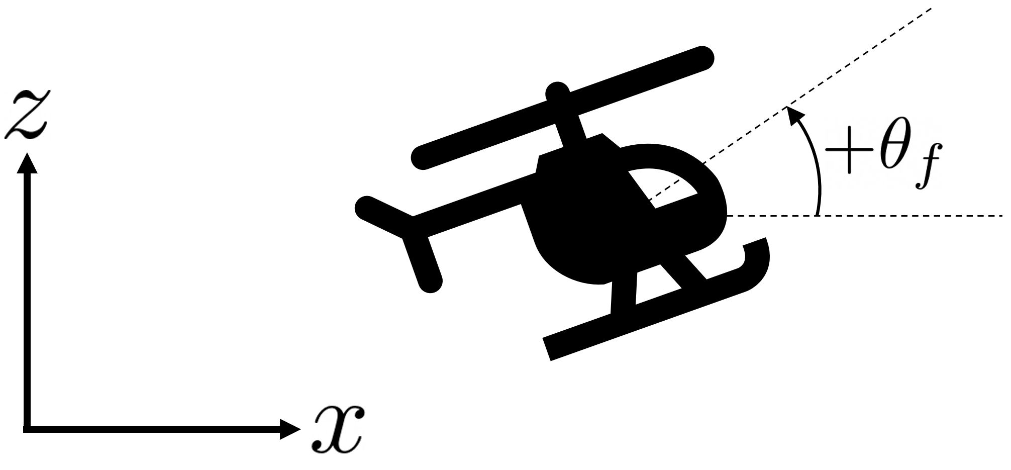
In the frame of reference we’re going to look at, the helicopter is constrained to motion in the $x-z$ plane, but it is not modeled as a particle: besides translating in the plane, the helicopter can change its pitch around the $y$ axis.

Helicopter Controls

In this simplified case, we can control the helicopter with two angular inputs: the collective pitch ${\theta }_0$ and the cyclic pitch ${\theta }_c$. When a pilot moves the cyclic control, it changes the pitch of the rotor blades at different points in their rotation. This allows the helicopter to tilt in the desired direction. In our three-degree-of-freedom case, this means the cyclic control is mainly responsible for setting the helicopter’s pitch ${\theta }_f$.

In contrast, the collective control adjusts the pitch of all the main rotor blades simultaneously. When the pilot raises the collective control, it increases the pitch of all rotor blades, generating more lift, which results in the helicopter ascending. Conversely, lowering the collective control decreases the pitch of the rotor blades, reducing lift and causing the helicopter to descend. In our three-degree-of-freedom case, this means the collective control is mainly responsible for setting the helicopter’s vertical position $z$.

Equations of Motion

There are some helicopter parameters that we need for the equations of motion. These are explained in Table 1 below.

Table 1: Helicopter parameters and values for the Sikorsky UH-60A.

Parameter	Symbol	UH-60A Value
Helicopter mass [kg]	$m$	4945
Moment of inertia ($y$-axis) [kg$\cdot$m${}^2$]	$I_y$	54233
Drag coeffient times frontal area [m${}^2$]	$C_{D}S$	1.26
Rotor rotational velocity [rad/s]	$\mathrm{\Omega }$	27
Rotor radius [m]	$R$	8.178
Rotor solidity [-]	$\sigma$	0.0821
Lift-curve slope, 2-dimensional [-]	$c_{l_{\alpha }}$	5.73
Lock number [-]	$\gamma$	8.1936
Height of the disk plane above the center of gravity [m]	$h$	1.6

Before going into the equations of motion, we can consider the main forces acting on the helicopter. These are the aircraft’s weight, the main rotor thrust, and the aerodynamic drag. The helicopter’s weight is straightforward; it’s simply $mg$ or its mass multiplicated by the Earth’s gravitational acceleration. The main rotor thrust can be expressed as:

$$\begin{array}{}\text{(1)}& T=C_T\rho (\mathrm{\Omega }R{)}^2\pi R^2,\end{array}$$ where $T$ is the thrust, $C_T$ is the thrust coefficient, and $\mathrm{\Omega }$ and $R$ are as defined in Table 1. The value of $C_T$ is determined iteratively using definitions from blade element theory and Glauert’s momentum theory.

On the other hand, the drag force $D$ is given by: $$\begin{array}{}\text{(2)}& D=C_D\frac{1}{2}\rho V^{2}S,\end{array}$$ where $V=\sqrt{u^2+v^2}$ is the magnitude of the helicopter’s velocity, $\rho$ is the air density, $C_D$ is the helicopter’s drag coefficient, and $S$ is its frontal surface area. The product $C_{D}S$ is assumed to be constant and is given in Table 1.

With the weight, thrust, and drag forces defined, we can go ahead and formulate the equations of motion for the three-degree-of-freedom helicopter. For the derivation of these equations, see [1].

First, we define the horizontal and vertical velocities $u$ and $v$ as the time derivatives of the helicopter’s $x$ and $z$ coordinates in Equation 3 and Equation 4: $$\begin{array}{}\text{(3)}& \dot{x}=u\end{array}$$

$$\begin{array}{}\text{(4)}& \dot{z}=w\end{array}$$

Similarly, we define the pitch rate $q$ as the time derivative of the helicopter’s pitch ${\theta }_f$ in Equation 5: $$\begin{array}{}\text{(5)}& {\dot{\theta }}_f=q\end{array}$$

Finally, Equation 6, Equation 7, and Equation 8 define the accelerations in all three of the model helicopter’s degrees of freedom: $$\begin{array}{}\text{(6)}& \dot{u}=-g\sin {\theta }_f-\frac{D}{m}\frac{u}{V}+\frac{T}{m}\sin ({\theta }_c-a_1)-qw\end{array}$$

$$\begin{array}{}\text{(7)}& \dot{w}=g\cos {\theta }_f-\frac{D}{m}\frac{w}{V}-\frac{T}{m}\cos ({\theta }_c-a_1)+qu\end{array}$$

$$\begin{array}{}\text{(8)}& \dot{q}=-\frac{T}{I_y}h\sin ({\theta }_c-a_1)\end{array}$$

In these last three equations, a new term shows up that we haven’t discussed: the rotor tilt angle $a_1$, or the longitudinal tilt of the rotor disc plane with respect to the control plane.

The Code

With our equations of motion, we can move on to actually solving them to carry out the simulation.

Imports

Let’s import some packages we’ll use down the line.

Code

from typing import Dict, Union

from matplotlib.collections import LineCollection
import matplotlib.pyplot as plt
import numpy as np
from scipy.integrate import solve_ivp
from scipy.optimize import fsolve

General Procedure

Following the steps outlined in [1], we can determine the equations of motion at a given time $t$ and advance a numerical scheme with that information. To achieve this, we need to define the following quantities for convenience:

• $V$, the magnitude of the helicopter’s velocity: $$\begin{array}{}\text{(9)}& V=\sqrt{u^2+w^2}\end{array}$$

• The angle of attack of the control plane ${\alpha }_c$: $$\begin{array}{}\text{(10)}& {\alpha }_c={\theta }_c-{\tan }^{-1}\left(\frac{w}{u}\right),\end{array}$$ where the inverse tangent is the two-argument arctangent.

• The advance ratio $\mu$: $$\begin{array}{}\text{(11)}& \mu =\frac{V}{\mathrm{\Omega }R}\cos {\alpha }_c\end{array}$$

• The non-dimensional inflow velocity of the control plane ${\lambda }_c$: $$\begin{array}{}\text{(12)}& {\lambda }_c=\frac{V\sin {\alpha }_c}{\mathrm{\Omega }R}\end{array}$$

Because we’re dealing with a system of differential equations with temporal derivatives, we can use the Runge-Kutta method to discretize the equations of motion and solve them iteratively.

Iterative Calculation of the Thrust Coefficient

Before solving the equations of motion, we need to take a look at how we can find the thrust coefficient $C_T$ that appears on Equation 1. The approach recommended in [1] is to find $C_T$ iteratively by reconciling the coefficients obtained via blade element theory and Glauert’s momentum theory. The formulas for these coefficients are:

$$\begin{array}{rl}{C}_{T,\text{BEM}}& =\frac{1}{4}{c}_{l_{\alpha }}\sigma [\frac{2}{3}{\theta }_0(1+\frac{3}{2}{\mu }^2)-({\lambda }_c-{\lambda }_i)]\\ C_{T,\text{Glauert}}& ={\lambda }_i\sqrt{{(\frac{V}{\mathrm{\Omega }R}\cos ({\alpha }_c-a_1))}^2+{(\frac{V}{\mathrm{\Omega }R}\sin ({\alpha }_c-a_1)+{\lambda }_i)}^2}\end{array}$$

Here, both definitions are connected by the non-dimensional induced velocity ${\lambda }_i$. As a result, we can find ${\lambda }_i$ such that $C_{T,\text{BEM}}=C_{T,\text{Glauert}}$. The rotor tilt angle $a_1$ that shows up in the definition for $C_{T,\text{Glauert}}$ also depends on ${\lambda }_i$ and is defined as:

$$\begin{array}{}\text{(13)}& a_1=\frac{-\frac{16q}{\gamma \mathrm{\Omega }}+\frac{8}{3}\mu {\theta }_0-2\mu ({\lambda }_c+{\lambda }_i)}{1-\frac{{\mu }^2}{2}}\end{array}$$

Code

def thrust_coefficient_residual(lambda_i: float, params: Dict[str, float]):
    """Calculate thrust coefficients and related parameters based on Blade Element
    Theory (BEM) theory and Glauert's momentum theory.

    Args:
        lambda_i (float):
            Inflow ratio, representing the ratio of axial velocity induced by the
            rotor to the free-stream velocity.
        params (Dict[str, float]):
            Dictionary containing aerodynamic parameters necessary for the calculations.
            The dictionary should include the following keys:
                - "gamma" (float): Lock number.
                - "q" (float): Pitch rate [rad/s].
                - "Omega" (float): Rotor angular velocity [rad/s].
                - "mu" (float): Advance ratio [-].
                - "theta_0" (float): Collective pitch angle [rad].
                - "lambda_c" (float): Non-dimensional inflow velocity of the control plane [-].
                - "cl_alpha" (float): Lift curve slope [rad^-1].
                - "sigma" (float): Solidity [-].
                - "alpha_c" (float): Angle of attack of the control plane [rad].
                - "V" (float): Helicopter speed [m/s].
                - "OmegaR" (float): Product of rotor angular velocity and rotor radius [m*rad/s].

    Returns:
        tuple:
            A tuple containing the following values:
                - The difference (residual) of the thrust coefficients calculated with both approaches.
                - Thrust coefficient based on BEM theory.
                - Thrust coefficient based on Glauert's correction.
                - Intermediate parameter 'a_1' used in the calculations.
    """

    # Calculate the rotor tilt angle
    a_1 = (
        (-16 / params["gamma"]) * (params["q"] / params["Omega"])
        + (8 / 3) * (params["mu"] * params["theta_0"])
        - 2 * params["mu"] * (params["lambda_c"] + lambda_i)
    ) / (1 - (1 / 2) * params["mu"] ** 2)

    # Blade element thrust coefficient
    thrust_coeff_BEM = (
        params["cl_alpha"]
        * (params["sigma"] / 4)
        * (
            (2 / 3) * params["theta_0"] * (1 + (3 / 2) * params["mu"] ** 2)
            - (params["lambda_c"] + lambda_i)
        )
    )

    # Glauert momentum thrust coefficient
    thrust_coeff_Glauert = (
        2
        * lambda_i
        * np.sqrt(
            (params["V"] * np.cos(params["alpha_c"] - a_1) / params["OmegaR"]) ** 2
            + (
                params["V"] * np.sin(params["alpha_c"] - a_1) / params["OmegaR"]
                + lambda_i
            )
            ** 2
        )
    )

    return (
        thrust_coeff_BEM - thrust_coeff_Glauert,
        thrust_coeff_Glauert,
        thrust_coeff_BEM,
        a_1,
    )

Now, we can define a lambda form to get only the first output of the thrust_coefficient_residual function above:

Code

target = lambda lambda_i, params: thrust_coefficient_residual(lambda_i, params)[0]

We’ll aim to find the root of this target function, thus getting the thrust coefficient we’re looking for and the angle $a_1$ that we need for the equations of motion. To do this, we’ll use SciPy’s fsolve, which finds the roots of a function given an initial guess. Let’s look at an example of how fsolve can help us find the thrust coefficient for a particular set of parameters. The dictionary sample_params will contain the values of the parameters needed for the calculation, and we’ll give an initial guess of ${\lambda }_i$ of 0.1. The result of calling fsolve will give us the value of ${\lambda }_i$ that ensures $C_{T,\text{BEM}}=C_{T,\text{Glauert}}$.

Code

sample_params = {
    "gamma": 8.1936,
    "q": 0.1,
    "Omega": 27,
    "mu": 0.25,
    "theta_0": 0.1,
    "lambda_c": 0.05,
    "cl_alpha": 0.1,
    "sigma": 0.08,
    "alpha_c": 0.08,
    "V": 5,
    "OmegaR": 27 * 8.178,
}

lambda_i = fsolve(target, 0.1, args=sample_params, xtol=1e-4)[0]

print(f'λ_i = {lambda_i:.3e}')

residual, c_t_glauert, c_t_bem, a_1 = thrust_coefficient_residual(lambda_i, sample_params)

print(f'C_T, Glauert = {c_t_glauert:.3e}')
print(f'C_T, BEM = {c_t_bem:.3e}')
print(f'a_1 = {a_1:.3f} rad = {np.rad2deg(a_1):.3f}°')

λ_i = 9.666e-04
C_T, Glauert = 4.390e-05
C_T, BEM = 4.390e-05
a_1 = 0.035 rad = 2.008°

With this example, we can see how fsolve helps us get the values for $C_T$ and $a_1$ used in the equations of motion that we’re trying to solve.

Numerical Solution of the Equations of Motion

Now, we’ll solve the system of six equations of motion (Equation 3 through Equation 8) to determine the path taken by the helicopter. To do this, we’ll take the system as an initial value problem and use SciPy’s solve_ivp.

The first step we need to take is to make a function in a format that works with solve_ivp’s signature. solve_ivp expects a function that gives the time derivatives of the form fun(t, y), where t (a scalar) is the time and y is an ndarray with all the state variables. In our helicopter case, the state variables are $x$, $u$, $z$, $w$, ${\theta }_f$, and $q$. As a result, we need to create a function that returns $\dot{x}$, $\dot{u}$, $\dot{z}$, $\dot{w}$, ${\dot{\theta }}_f$, and $\dot{q}$ in a single ndarray. We also need to provide our function with the control variables ${\theta }_0$ and ${\theta }_c$ and with the helicopter parameters that show up in the drag and thrust calculations. The code for this function is shown below.

Code

def derivatives(
    t: float,
    y: Union[list, np.ndarray],
    theta_0: float,
    theta_c: float,
    aircraft_parameters: dict,
) -> list:
    """
    Function that determines the 3-DoF helicopter's equations of motion
    Args:
        t (float): Current time
        y (Union[list, np.ndarray]): State vector [x, u, z, w, theta_f, q]^T
        theta_0 (float): Control action on collective pitch
        theta_c (float): Control action on cyclic pitch
        aircraft_parameters (dict): Dictionary with helicopter's parameters

    Returns:
        list: dy/dt vector
    """
    # Unpack the state vector y
    x, u, z, w, theta_f, q = y

    # Calculate velocity magnitude
    V = np.sqrt(u**2 + w**2)

    # Calculate the parameter alpha_c
    if u == 0:
        alpha_c = np.pi / 2
    else:
        alpha_c = -np.arctan(w / u) + theta_c

        if u < 0:
            alpha_c += np.pi

    # Calculate the parameter mu
    mu = (V / (aircraft_parameters["Omega"] * aircraft_parameters["R"])) * np.cos(
        alpha_c
    )
    # Calculate the parameter lambda_c
    lambda_c = (V / (aircraft_parameters["Omega"] * aircraft_parameters["R"])) * np.sin(
        alpha_c
    )

    # Parameter dictionary for thrust coefficient calculation
    params = {
        **aircraft_parameters,
        "OmegaR": aircraft_parameters["Omega"] * aircraft_parameters["R"],
        "q": q,
        "mu": mu,
        "theta_0": theta_0,
        "lambda_c": lambda_c,
        "alpha_c": alpha_c,
        "V": V,
    }

    # Determine the correct induced velocity lambda_i by iteratively making
    # C_T_Glauert and C_T_elem equal
    lambda_i = fsolve(target, 0.1, args=params, xtol=1e-4)[0]

    # Get the correct thrust coefficient and a_1 parameter with the lambda_i calculated above
    _, C_T, _, a_1 = thrust_coefficient_residual(lambda_i, params)
    # Calculate dimensional thrust
    T = (
        C_T
        * aircraft_parameters["rho"]
        * (aircraft_parameters["Omega"] * aircraft_parameters["R"]) ** 2
        * np.pi
        * aircraft_parameters["R"] ** 2
    )
    # Calculate dimensional drag
    D = aircraft_parameters["CD_S"] * 0.5 * aircraft_parameters["rho"] * V**2

    # Longitudinal acceleration
    u_dot = (
        -aircraft_parameters["g"] * np.sin(theta_f)
        - (D * u) / (aircraft_parameters["M"] * V)
        + (T / aircraft_parameters["M"]) * np.sin(theta_c - a_1)
        - q * w
    )
    # Vertical acceleration
    w_dot = (
        aircraft_parameters["g"] * np.cos(theta_f)
        - (D * w) / (aircraft_parameters["M"] * V)
        - (T / aircraft_parameters["M"]) * np.cos(theta_c - a_1)
        + q * u
    )

    # Angular (pitch) acceleration
    q_dot = (
        -(T / aircraft_parameters["I_y"])
        * aircraft_parameters["h"]
        * np.sin(theta_c - a_1)
    )

    # Vector of derivatives:
    #       x_dot, u_dot, z_dot, w_dot, theta_f_dot, q_dot
    y_dot = [u, u_dot, w, w_dot, q, q_dot]

    return y_dot

Now, we can solve the equations of motion given initial values for our state variables at $t=0$. Some example values are given in Table 2.

Table 2: Initial state variable values for the helicopter simulation.

$x_0$ [m]	$u_0$ [m/s]	$z_0$ [m]	$w_0$ [m/s]	${\theta }_{f_0}$ [°]	$q_0$ [°/s]
-10	5	10	0	-1	0

For our first simulation, we’ll just take constant values of the control variables ${\theta }_0$ and ${\theta }_c$. We’ll take ${\theta }_0=6^{\circ }$ and ${\theta }_c=1^{\circ }$ and see what happens over a simulation time of 30 seconds.

Code

aircraft_parameters = {
    "Omega": 27,  # Angular velocity of the rotor (in rad/s)
    "R": 8.178,  # Rotor radius (in meters)
    "gamma": 8.1936,  # Ratio of specific heats
    "cl_alpha": 5.73,  # Lift curve slope (per rad)
    "sigma": 0.08210,  # Solidity of the rotor
    "CD_S": 1.26,  # Drag coefficient times reference area
    "rho": 1.225,  # Air density (in kg/m^3)
    "M": 4945,  # Mass of the helicopter (in kg)
    "I_y": 54233,  # Moment of inertia about the y-axis (in kg*m^2)
    "h": 1.6,  # Distance from the rotor to the center of mass (in meters)
    "g": 9.81,  # Acceleration due to gravity (in m/s^2)
}

# Initial state variables: [x0, u0, z0, w0, θ_f0, q0]
y_0 = np.array([-10, 5, 10, 0, -1, 0])

solution = solve_ivp(
    fun=derivatives,
    t_span=[0, 30],
    y0=y_0,
    method="BDF",
    args=(np.deg2rad(6), np.deg2rad(1), aircraft_parameters),
    max_step=0.1,
)

Let’s visualize the helciopter’s trajectory. To do this, we’ll extract some information from the solution object returned by solve_ivp.

Code

points = np.vstack((solution.y[0, :], solution.y[2, :])).T.reshape(-1, 1, 2)
segments = np.concatenate([points[:-1], points[1:]], axis=1)

fig, ax = plt.subplots()
norm = plt.Normalize(min(solution.t), max(solution.t))
lc = LineCollection(segments, cmap="viridis", norm=norm)
lc.set_array(solution.t)
line = ax.add_collection(lc)
fig.colorbar(line, ax=ax, label="Time [s]")
ax.set_xlim(-50, max(solution.y[0, :]) * 1.05)
ax.set_ylim(min(solution.y[2, :]) * 1.05, max(solution.y[2, :]) * 1.05)
ax.set_xlabel("$x$ [m]")
ax.set_ylabel("$z$ [m]")
ax.set_title("Helicopter trajectory")
plt.show()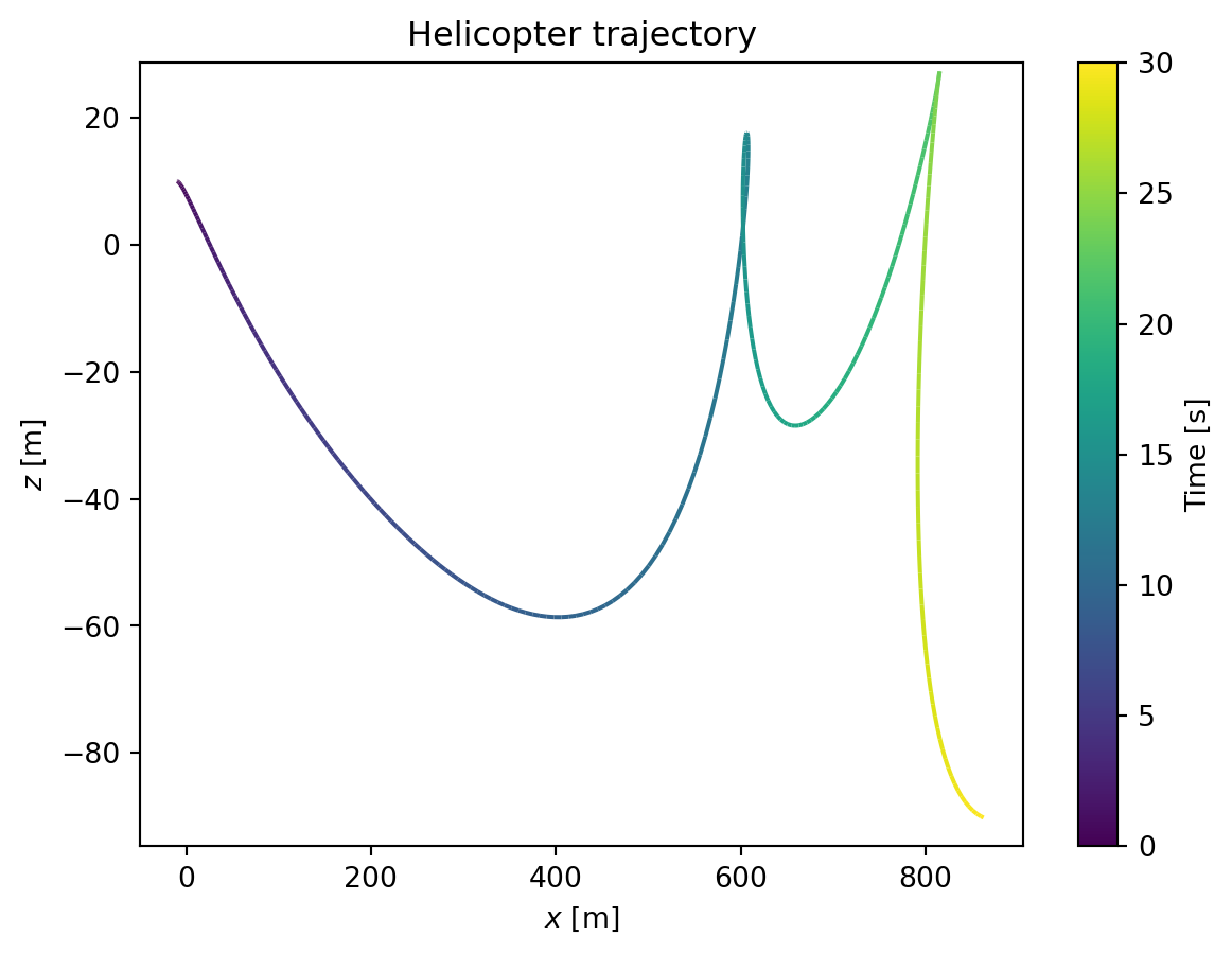

Figure 2: The helicopter’s trajectory under constant collective and cyclic pitches.

Figure 2 shows the result. It looks like a pretty rough ride! We see lots of vertical oscillation and a very sudden downward plunge towards the end of the simulation. We would be better off selecting our control variables more carefully. We’ll do just that in a future post. For now, we’ve successfully shown how to simulate a three-degree-of-freedom helicopter model by solving its equations of motion.

References

[1]

van Holten, T., and Melkert, J. A., “Helicopter Performance, Stability and Control,” Delft University of Technology, Delft, The Netherlands, 2002.